Natural Deduction

Natural Deduction (ND) is a common name for the class of proof systems composed of simple and self-evident inference rules based upon methods of proof and traditional ways of reasoning that have been applied since antiquity in deductive practice. The first formal ND systems were independently constructed in the 1930s by G. Gentzen and S. Jaśkowski and proposed as an alternative to Hilbert-style axiomatic systems. Gentzen introduced a format of ND particularly useful for  theoretical investigations of the structure of proofs. Jaśkowski instead provided a format of ND more suitable for practical purposes of proof search. Since then many other ND systems were developed of apparently different character.

What is it that makes them all ND systems despite the differences in the selection of rules, construction of proof, and other features? First of all, in contrast to proofs in axiomatic systems, proofs in ND systems are based on the use of assumptions which are freely introduced but discharged under some conditions. Moreover, ND systems use many inference rules of simple character which show how to compose and decompose formulas in proofs. Finally, ND systems allow for the application of different proof-search strategies. Thanks to these features proofs in ND systems tend to be much shorter and easier to construct than in axiomatic or tableau systems. These properties of ND make them one of the most popular ways of teaching logic in elementary courses. In addition to its educational value, ND is also an important tool in proof-theoretical investigations and in the philosophy of meaning (specifically, of the meaning of logical constants). This article focuses on the description of the main types of ND systems and briefly mentions more advanced issues concerning normal proofs and proof-theoretical semantics.

Table of Contents

1. History of Natural Deduction
   1. Origins
   2. Prehistory
2. Applications
3. Demarcation Problem
   1. Wide and Narrow Sense of ND
   2. Criteria of Genuine ND
4. Rules
5. Proof Format
   1. Tree Proofs
   2. Linear Proofs
6. Other Approaches
7. Rules for Quantifiers
8. ND for Non-Classical Logics
9. Normal Proofs
10. Philosophy of Meaning
11. References and Further Reading

1. History of Natural Deduction

When dealing with the history of ND, one should distinguish between the exact date when the first formal systems of ND were presented and much earlier times when the rules of ND were actually applied. Although one may claim that ND techniques were used as early as people did reasoning, it is unquestionable that the exact formulation of ND and the justification of its correctness was postponed until the 20th century.

a. Origins

The first ND systems were developed independently by Gerhard Gentzen and Stanisław Jaśkowski and presented in papers published in 1934 (Gentzen 1934, Jaśkowski 1934). Both approaches, although different in many respects, provided the realization of the same basic idea: formally correct systematization of traditional means of proving theorems in mathematics, science and ordinary discourse. It was a reaction to the artificiality of formalization of proofs in axiomatic systems. Hilbert’s proof theory offered high standards of precise formulation of this notion, but formal axiomatic proofs were really different than ‘real’ proofs offered by mathematicians. The process of actual deduction in axiomatic systems is usually complicated and needs a lot of invention. Moreover, real proofs are usually lengthy, hard to decipher and far from informal arguments provided by mathematicians. In informal proofs, techniques such as conditional proof, indirect proof or proof by cases are commonly used; all are based on the introduction of arbitrary, temporarily accepted assumptions. Hence the goals of Gentzen and Jaśkowski were twofold: (1) theoretical and formally correct justification of traditional proof methods, and (2) providing a system which supports actual proof search. Moreover, Gentzen’s approach provided the programme for proof analysis which strongly influenced modern proof theory and philosophical research on theories of meaning.

b. Prehistory

According to some authors the roots of ND may be traced back to Ancient Greece. Corcoran (1972) proposed an interpretation of Aristotle’s syllogistics in terms of inference rules and proofs from assumptions. One can also look for the genesis of ND system in Stoic logic, where many researchers (for example, Mates 1953) identify a practical application of the Deduction Theorem (DT). But all these examples, even if we agree with the arguments of historians of logic, are only examples of using some proof techniques. There is no evidence of theoretical interest in their justification.

In fact the introduction of DT into the realm of modern logic seems to be one of the most important steps on the way leading eventually to the discovery of ND. Although Herbrand did not present a formal proof of it for axiomatic systems until Herbrand (1930), he had already stated it in Herbrand (1928). At the same time Tarski (1930) included DT as one of the axioms of his Consequence Theory; in practice he had used it since 1921. Also other ND-like rules were practically applied in the 1920s by many logicians from the Lvov-Warsaw School, like Leśniewski and Salamucha, as is evident from their papers.

Jaśkowski was strongly influenced by Łukasiewicz, who posed on his Warsaw seminar in 1926 the following problem: how to describe, in a formally proper way, proof methods applied in practice by mathematicians. In response to this challenge Jaśkowski presented his first formulation of ND in 1927, at the First Polish Mathematical Congress in Lvov, mentioned in the Proceedings (Jaśkowski 1929). A final solution was delayed until (Jaśkowski 1934) because Jaśkowski had a lengthy break in his research due to illness and family problems. Gentzen also published the first part of his famous paper in 1934, but the first results are present in (Gentzen 1932). This early paper, however, is concerned not with ND but with the first form of Sequent Calculus (SC). Gentzen was influenced by Hertz (1929), where a tree-format notation for proofs, as well as the notion of a sequent, were introduced. One can also look for a source of the shape of his rules in Heyting’s axiomatization of intuitionistic logic (see von Plato 2014).

It should be no surprise that the two logicians with no knowledge of each other’s work, independently proposed quite different solutions to the same problem. Axiom systems, although theoretically satisfying, were considered by many researchers as practically inadequate and artificial. Thus the need for more practice-oriented deduction systems was in the air.

2. Applications

This article distinguishes at least three main fields of application of ND systems: practical, theoretical and philosophical.

Since 1934 a lot of systems called ND were offered by many authors in numerous textbooks on elementary logic. In this way ND systems became a standard tool of working logicians, mathematicians, and philosophers. At least in the Anglo-American tradition, ND systems prevail in teaching logic. They also had strong influence on the development of other types of non-axiomatic formal systems such as sequent calculi and tableau systems. In fact, the former were also invented by Gentzen as a theoretical tool for investigations on the properties of ND proofs, whereas the latter may be seen (at least in the case of classical logic) as a further simplification of sequent calculus that is easier for practical applications.

But the importance of ND is not only of practical character. Since 1960s the works of Prawitz (1965) and (Raggio 1965) on normal proofs opened up the theoretical perspective in the applications of ND. In fact Prawitz was rediscovering things known to Gentzen but not published by him, which was later shown by von Plato (2008). In addition to extended work on normalization of proofs, ND is also an interesting tool for investigations in theoretical computer science through the Curry-Howard isomorphism. This approach shows that (normal) ND proofs may be interpreted in terms of executions of programs.

Finally the special form of rules of ND provided by Gentzen led to extensive studies on the meaning of logical constants. This article takes a look at theoretical and philosophical applications of ND in sections 9 and 10.

3. Demarcation Problem

The great richness of different forms of systems called ND leads to some theoretical problems concerning the precise meaning of the term ‘ND’. It seems that no definition of ND systems was offered which would be generally accepted. This demarcation problem was investigated by many authors; and different criteria were offered for establishing what is, and what is not, an ND system. Detailed survey of these matters may be found in Pelletier (1999) or in Pelletier and Hazen (2012); this article points out only the most important features.

a. Wide and Narrow Sense of ND

Some authors tend to use the term in a broad sense in which it covers almost all that is not an axiomatic system in Hilbert’s sense. Hence sometimes systems like sequent calculi or tableau calculi are treated as ND systems. All these systems are actually in close relationship, but this article chooses to consider ND only in the narrow sense. There are at least three reasons for making this choice:

• Historical. Original ideas of Gentzen, who introduced two systems: NK (Natürliche Kalkül) and LK (Logistiche Kalkül). The former is just an ND system, whereas the latter, a sequent calculus, was meant as a technical tool for proving some metatheorems on NK, not as a kind of ND.
• Etymological. ND is supposed to reconstruct, in a formally proper way, traditional ways of reasoning. It is disputable whether existing ND systems realize this task in a satisfying way, but certainly systems like tableaux or SC are even worse in this respect.
• Practical. Taking the term ND in a wide sense would be a classifying operation of doubtful usefulness. From the point of view of this article’s presentation, it is more convenient to use a more narrowly defined concept.

b. Criteria of Genuine ND

But what criteria should be used for delimiting the class of systems called ND? Many proposals seem to be too narrow (that is, strict) since they exclude some systems usually treated as ND, so it is better not to be very demanding in this respect. So, ND system should satisfy three criteria:

1. Possibility of entering and eliminating (discharging) additional assumptions during the course of the proof. Usually it requires some bookkeeping devices for indicating the scope of an assumption, that is, for showing that a part of the proof (a subproof) depends on a temporary assumption, and for marking the end of such a subproof the point at which the assumption is “discharged”.
2. Characterization of logical constants by means of rules rather than axioms. Their role is taken over by the set of primitive rules for introduction and elimination of logical constants, which means that elementary inferences instead of formulas are taken as primitive.
3. The richness of forms of proof construction. Genuine ND systems admit a lot of freedom in proof construction and in the possibility of applying several strategies of proof-search.

These three conditions seem to be the essential features of any ND. These characteristics are quite general, but the third at least serves to exclude tableau systems and sequent calculi since genuine ND should allow both direct and indirect proofs, proofs by cases, and so forth. This flexibility of proof construction is vital for ND, whereas, for example in a standard tableau system, we have only indirect proofs and elimination rules. On the other hand, ND does not require that its rules should strictly realise the schema of providing a pair of introduction and elimination rules, and that axioms are not allowed.

4. Rules

ND systems consist of the set of (schemata) of simple rules characterising logical constants. For example a connective of conjunction is characterised by means of the following rules:

   

where and denote any formulas. Material above the horizontal line represents the premises; and that below represents the conclusion of the inference. The letters and in the names of the rules come from “introduction” and “elimination” respectively since the first allows introduction of a conjunction into a proof, and the second allows for its elimination in favor of simpler formulas. Often the following horizontal notation is applied (instead of vertical which is more space-consuming):

   

Here is used to point out that the relation of deducibility holds between premises and the conclusion of a rule instance. In what follows, such phrases are called sequents. In fact such deducibility statements in general do not uniquely characterise inference rules, but it does no harm so they are used in what follows for simplicity’s sake.

One can easily check that the rules stated above adequately characterise the meaning of classical conjunction which is true iff both conjuncts are true. Hence the syntactic deducibility relation coincides with the semantic relation of , that is, of logical consequence (or entailment). Unfortunately not all logical constants may be characterised by means of such simple rules. For example, implication in addition to modus ponens (or detachment rule):

   

which is known from axiomatic systems, requires a more complex rule of the shape:

   

or:

 
where and forms a collection of all active assumptions previously introduced which could have been used in the deduction of . When inferring , one is allowed to discharge assumptions of the form . The fact that after deduction of this assumption is discharged (not active) is pointed out by using [ ] in vertical notation, and by deletion from the set of assumptions in horizontal notation. The latter notation shows better the character of the rule; one deduction is transformed into the other. It shows also that the rule corresponds to an important metatheorem, the Deduction Theorem, which has to be proved in axiomatic formalizations of logic. In what follows, all rules of the shape will be called inference rules, since they allow for inferring a formula (conclusion) from other formulas (premises) present in the proof. Rules of the form:

 
will be called proof construction rules since they allow for constructing a proof on the basis of some proofs already completed. One characteristic feature of such rules is that they involve the process of entering new assumptions as well as conditions under which one can discharge these assumptions and close subordinated proofs (or subproofs) starting with these assumptions.

The complete set of rules provided by Gentzen for IPL (Intuitionistic Propositional Logic) is the following:

   

What is evident from this set of rules is the Gentzen policy of characterising every constant by a pair of rules, in which one is the rule for introduction a formula with that constant into a proof, and the other is the rule of elimination of such a formula, that is, inferring some simpler consequences from it, sometimes with the aid of other premises. More will be said about philosophical consequences of this approach in section 10.

In order to obtain CPL (Classical Propositional Logic), Gentzen added the Law of Excluded Middle as an axiom, but the same result can easily be obtained by a suitable inference rule of double negation elimination: or by changing one of the proof construction rules, namely ) which encodes the weak form of indirect proof into the strong form:

 
This solution was applied by Jaśkowski (1934).

5. Proof Format

In addition to providing suitable rules, one must also decide about the form of a proof. Two basic approaches due to Gentzen and Jaśkowski are based on using trees as a representation of a proof and on using linear sequences of formulas. This article focuses on the most important differences between these two approaches. For detailed comparison see Pelletier and Hazen (2014), and Restall (2014).

a. Tree Proofs

Let us start with an example of a proof in Gentzen’s format, that is, as a tree of formulas:

   

Here the root of a tree is labelled with a thesis and its leaves are labelled with (discharged) assumptions: and . All assumptions were discharged while was applied successively building implications from — the numbers of assumptions indicate the order in which they were discharged, and the suitable number is attached to the formula inferred by the assumption discharging rule. Before that, was deduced by two applications of , first to two assumptions (active at this moment), then to the third assumption and previously deduced .

Gentzen’s tree format of representing proofs has many advantages. It is an excellent representation of real proofs; in particular, deductive dependencies between formulas are directly shown. But if we are concerned with actual deduction, this format of proof is far from being useful and natural. Moreover, one is often forced to repeat identical, or very similar, parts of the proof, since, in tree format, inferences are conducted not on formulas but on their particular occurrences. For example, if is an assumption from which we need to infer both and , then a suitable branch starting with must be displayed twice. The following example illustrates the point:

   

here, the attachment of two numerals to the formula in the last line indicates that both occurrences of the same assumption were discharged in this step.

Gentzen himself was aware of the disadvantages of his representation of proof, but it proved useful for his theoretical interests described in section 9. It is not surprising that the tree format of proofs is mainly used in theoretical studies on ND, as in Prawitz (1965) or Negri and von Plato (2001).

b. Linear Proofs

Jaśkowski, on the other hand, preferred a linear representation of proofs since he was interested in creating a practical tool for deduction. Linear format has many virtues over Gentzen’s approach. For example, inferences are drawn from assumptions rather than from their occurrences, which means that, for example, one needs to assume only once to derive both conjuncts. It is also more natural to construct a linear sequence trying, one by one, each possible application of the rules. But there is a price to be paid for these simplifications—the problem of subordinated proofs. How should we represent that some assumption and its subordinated proof are no longer alive because a suitable proof construction rule was applied? If we apply a proof construction rule which discharges an assumption, we must explicitly show that the subordinate proof dependent on this assumption is dead in the sense that no formula from it may be used below in the proof. In a tree format this is not a problem—to use a formula as a premise for the application of some inference rule we must display it (and the whole subtree which provides a justification for it) directly above the conclusion. In linear format this leads to problems, and some technical devices are necessary which forbid using the assumptions and other formulas inferred inside completed subproofs. Jaśkowski proposed two solutions to this problem: graphical (boxes) and bookkeeping (in the terminology of Pelletier and Hazen 2012). Let us compare these two simple proofs:

 

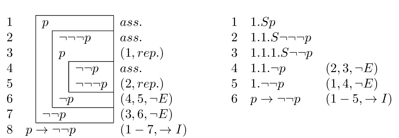
On the left we have an example of a proof in graphical mode where each assumption opens a new box in which the rest of the proof is carried out. On the other hand when a suitable proof construction rule is applied, the current subproof is boxed which means that nothing inside is allowed in further proof construction. In lines 3 and 5 an additional rule of repetition (often called reiteration) is applied which allows for moving formulas from outer to inner boxes. On the right the same proof is represented in bookkeeping style where instead of boxes we use prefixes (sequences of natural numbers) for indicating the scope of an assumption. Each assumption is preceded with the letter S from latin suppositio and adds a new numeral to the sequence of natural numbers in the prefix. When a proof construction rule is applied, the last item is subtracted from the prefix. Hence a thesis can occur with an empty sequence, signifying that it does not depend on any assumption. No repetition rules are applied in this version of Jaśkowski’s system; hence the proof is two lines shorter.

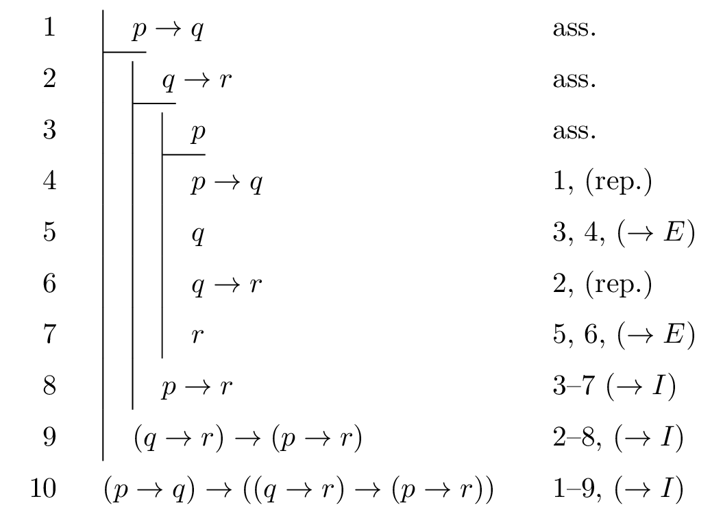
Although Jaśkowski finally chose the second option (perhaps due to editorial problems) nowadays the graphical approach is far more popular, probably due to the great success of Fitch’s textbook (1952) which popularized a simplified version of Jaśkowski’s system (now called Fitch’s approach). In Fitch’s system one is using vertical lines for indicating subproofs. Below is an example of a proof in Fitch’s format:

 

Other devices were also applied such as brackets in Copi (1954), or even just indentation of subordinate proofs. The original Jaśkowski’s boxes were used by Kalish and Montague (1964) with the additional device being of great heuristic value; each box is preceded by a show-line which displays the current aim of the proof. Show-lines are not parts of a proof in the sense that one is forbidden to use them as premises for rule application. But after completing a subproof, a box is closed and the opening show-line becomes a new ordinary line in the proof (which is pointed out by deleting a prefix “show”).

The second solution of Jaśkowski was not so popular. One can mention here Quine’s system (1950) (with asterisks instead of numerals) or Słupecki and Borkowski’s system (1958) popular in Poland.

6. Other Approaches

Gentzen (1936) introduced yet another variant of ND which may be considered as lying between his first system described in subsection 5.1. and his famous sequent calculus. It shows another possible way of arranging the bookkeeping of active assumptions. As a result, in this approach the basic items which are transformed in proofs are not formulas but rather sequents. For example, both rules for conjunction are of the form:

   

where are records of active assumptions.

The full list of rules for CPL contains also:

   

Assumptions are sequents of the form . Theses are sequents with an empty antecedent. Here is an example of a proof:

   

One can observe that in the context of such a system the difference between inference and proof construction rules disappears. The only difference is that in the former all transformations are performed on consequents of sequents whereas in the latter some operations (that is, subtractions) are allowed also on antecedents. This is the difference with Gentzen’s ordinary sequent calculus where we have rules introducing constants to antecedents of sequents (instead of rules of elimination). Of course one can go further and allow this kind of rule as well (such a system was constructed, for example, by Hermes 1963), but it seems that Gentzen’s choice offers significant simplifications. First of all, the tree format is not necessary, and one can display proofs as linear sequences since the record of active assumptions is kept with every formula in a proof (as the antecedent). Moreover, since no operation except subtraction is carried out on antecedents, we can get rid of formulas in antecedents and use instead numerals of lines where suitable assumptions were introduced into proofs. Both simplifications are present in Suppes’ system (1957) of ND where the same proof looks like that:

   

Other solutions generalising standard proof representations were also considered. One can mention at least two approaches without going into details: ND operating on clauses instead of formulas (Borićić 1985, Cellucci 1992, Indrzejczak 2010)  and ND admitting subproofs as items in the proof (Fitch 1966, Schroeder-Heister 1984).

7. Rules for Quantifiers

Gentzen (1934) also provided the first set of ND rules adequate for CFOL (Classical First-Order Logic) whereas the rules of Jaśkowski’s system characterised the weaker system of IFOL (Inclusive First-Order Logic) which admits empty domains in models. As pointed out by Bencivenga (2014), a minimal relaxation of Jaśkowski’s rules yields also Free Logic, that is, a logic allowing non-denoting terms, hence it may be claimed that it is the first formalization of Universally Free Logic, that is, allowing both empty domains and non-denoting terms.

Before characterising Gentzen’s original rules for quantifiers let us note that he was using two sorts of symbols to distinguish between free and bound individual variables. The former are often called individual parameters. Such a solution simplifies a formulation of rules and eliminates the risk of a clash of variables while applying the rules. When we provide ND rules for more standard approaches with just individual variables which may have free or bound occurrences, we must be careful to define precisely the operation of proper substitution of a term for all free occurrences of a variable. ‘Proper’ means that no occurrence of a free variable substituted for another (or, when function-symbols are used, within a term substituted for a variable) gets bound by a quantifier. For simplicity’s sake we will keep Gentzen’s solution; let denote (bound) variables and free variables or individual parameters. Gentzen’s rules are the following:

   

where [x/a] denotes the operation of substitution, that is, of replacing all free occurrences of in with a parameter . In case of and a parameter is required to be “fresh” in the sense of having no other occurrences in . Such a fresh is sometimes called an ‘eigenvariable’ or a ‘proper variable’.

The last rule in Gentzen’s tree format looks as follows:

   

Although Gentzen provided this set of rules for his tree-system of ND, it was easily adapted also to linear systems based on Jaśkowski’s (or Suppes’) format of proof. Let us illustrate their application in Fitch’s proof format (but not with his original rules):

 

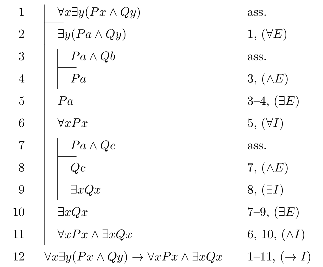
The first application of introduces a parameter in place of . In line 3 and 7 the assumptions for the applications of in line 5 and 10 respectively are introduced, each time with a new eigenparameter in place of . Note that both applications of are correct since neither nor are present in the formulas ending suitable subproofs. Also the application of in line 6 is correct since is not present in line 1.

The fact that ) is a proof construction rule is obscured here since there is no need to introduce a subproof by means of a new assumption. We just require that in order to apply there be no occurrence of an involved parameter (here ) in active assumptions. However, there are systems of ND where such a subproof (usually flagged with a fresh parameter which will be universally quantified below) is explicitly introduced into a proof. For instance, the original Fitch’s rule is based on such a solution; in fact it follows closely the original Jaśkowski’s rule for inclusive general quantifier.

Gentzen’s was sometimes considered as complex and artificial, and some inference rules were proposed instead where is directly inferred and not assumed. Although the idea is simple its correct implementation leads to troubles. Carefull formulations of such a rule (as in Quine 1950) are correct but hard to follow; simple formulations (as in several editions of Copi 1954) make the system unsound. For a detailed analysis of the relations between Gentzen-style and Quine-style quantifier rules one should consult Fine (1985), Hazen (1987) and Pelletier (1999). All these problems with providing correct and simple rules for quantifiers led some authors to doubt if it is really possible (see Anellis 1991). It seems that the only correct system of ND for CFOL with ‘really’ simple rule of this kind is in Kalish and Montague (1964), but this is rather a side-effect of the overall architecture of the system which is not discussed here (but see a detailed explanation of the virtues of Kalish and Montague’s system in Indrzejczak 2010).

8. ND for Non-Classical Logics

ND systems were also offered for many important non-classical logics. In particular, Jaśkowski’s graphical approach is very handy in this field due to the machinery of isolated subproofs. It appeared that for many non-classical logics one can obtain a satisfying result by putting restrictions on the rule of repetition in the case of some subproofs. Let us take as an example the ND formalization of well known propositional modal logic T; for simplicity we restrict considerations to rules for (necessity). is obvious: . With the situation is more complicated since it is based on the following principle:

 
where formulas in the antecedent are also being changed by addition of . It is realised by means of a special ‘modal’ subproof which is opened with no assumption, but no other formulas may be put in it except those which were preceded by in outer subproofs (and with deleted after transition). If in such modal subproof we deduce , it can be closed and can be put into the outer subproof. The following proof in Fitch’s style illustrates this:

 

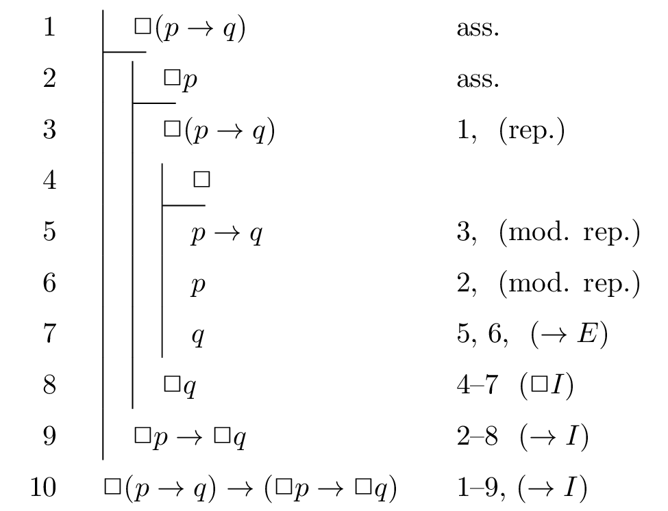
In line 4 a modal subproof was initiated which is shown by putting a sole in place of the assumption. Lines 5 and 6 result from the application of modal repetition. Such an approach may be easily extended to other modal logics by modifying conditions of modal repetition; for example, for S4 it is enough to admit that formulas with (no deletion) also may be repeated; for S5, formulas with negated are also allowed. Such an approach to modal logics was initiated by Fitch (1952), extensive study of such systems can be found in Fitting (1983), Garson (2006) and Indrzejczak (2010) where also some other approaches are discussed.

This modus of formalizing logics in ND was also applied for other non-classical logics including conditional logics (Thomason 1970), temporal logics (Indrzejczak 1994) and relevant logics (Anderson and Belnap 1975). In the latter the technique of restricted repetition is not enough however (and even not required for some logics of this kind). Far more important is the technique of labeling all formulas with sets of numbers annotating active assumptions which is necessary for keeping track of relevance conditions. Subsequently, applications of labels of different kinds is in fact one of the most popular technique used not only in tableau methods but also in ND. Vigano (2000) provides a good survey of this approach.

9. Normal Proofs

When constructing proofs one can easily make some inferences which are unnecessary for obtaining a goal. Gentzen was interested not only in providing an adequate system of ND but also in showing that everything which may be proved in such a system may be proved in the most straightforward way. As he put it, in such a proof “No concepts enter into the proof other than those contained in its final result, and their use was therefore essential to the achievement of the result’’ (Gentzen 1934).

In particular, such unnecessary moves are performed if one first applies some introduction rule for logical constant and then uses the conclusion of this rule application as a premise for the application of the elimination rule for . In such cases the final conclusion is either already present in the proof (as one of the premises of respective introduction rule) or may be directly deduced from premises of the application of introduction rule. For example, if one is deducing on the basis of and then by is deducing from this implication and , then it is simpler to deduce directly from ; the existence of such a proof is guaranteed because it is a subproof introducing . Let us call a maximal formula any formula which is at the same time the conclusion of an introduction rule and the main premise of an elimination rule. A proof is called normal iff no maximal formula is present in it. Roughly speaking we can obtain such a proof if first we apply elimination rules to our assumptions (premises) and then introduction rules to obtain the conclusion. Such proofs are analytic in the sense of having the subformula property: all formulas occurring in such a proof are subformulas or negations of subformulas of the conclusion or premises (undischarged assumptions).

Although the idea of a normal proof is rather simple to grasp it is not so simple to show that everything provable in ND system may have a normal proof. In fact for many ND systems (especially for many non-classical logics) such a result does not hold. Gentzen proved such a result directly for an ND system for Intuitionistic Logic, but he was unable to provide a proof for his ND for Classical Logic. He failed to provide the proof for the Intuitionistic case and instead he provided the result for both his ND systems indirectly. First he introduced an auxiliary technical system of sequent calculus and proved for it (both in the classical and intuitionistic cases) the famous Cut-Elimination Theorem. Then he showed that this result implies the existence of a normal proof for every thesis and valid argument provable in his ND systems. Such a result is usually called the Normal Form Theorem whereas the stronger result showing directly how to transform every ND-proof into normal proof by means of a systematic procedure is called the Normalization Theorem. That Gentzen indeed proved the Normalization Theorem for Intuitionistic case became known recently due to von Plato (2008) who found a preliminary draft of Gentzen’s thesis. The first published versions of proofs of Normalization theorems appeared in the 1960s due to Raggio (1965) and Prawitz (1965) who proved this result also for ND systems for some non-classical logics. For a detailed account of these problems see Troelstra and Schwichtenberg (1996) or Negri and von Plato (2001).

One thing should be noticed with respect to proofs in normal form. Although normal proofs are in a sense the most direct proofs, this does not mean that they are the most economical. In fact, non-normal proofs often may be shorter and easier to understand than normal ones. Perhaps it is simpler to understand if we recall that normalization in ND is the counterpart of cut-elimination in sequent calculi. Applications of cuts in proofs correspond to applications of previously proved things as lemmas and may drastically shorten proofs. When a proof is normalized, its size may grow exponentially (see, for example, Boolos 1984, Fitting 1996, D’Agostino 1999). What is important in normal proofs is that, due to their conceptual simplicity, they provide a proof theoretical justification of deduction and a new way of understanding the meaning of logical constants.

10. Philosophy of Meaning

Aesthetics was not the only reason for insisting on having both introduction and elimination rules for every constant in Gentzen’s ND. He also wanted to realise a deeper philosophical intuition concerning the meaning of logical constants. It is claimed that if a set of rules is intuitive and sufficient for adequate characterisation of a constant, then it in fact expresses our way of understanding this constant. Moreover, such an approach may be connected with Wittgenstein’s program of characterization of meaning by means of the use of words. In this particular case the meaning of logical constants is characterised by their use (via rules) in proof construction. There is also a strong connection with anti-realistic position in the philosophy of meaning where it is claimed that the notion of truth may be successfully replaced with the notion of a proof (Dummett 1991). One recent, and very strong, version of this trend is represented in Brandom’s (2000) program of strong inferentialism, where it is postulated that the meanings of all expressions may be characterised by means of their use in widely understood reasoning processes. However, inferentialism is not particularly connected with ND nor with the specific shapes of rules as giving rise to the meaning of logical constants.

Leaving aside the far-reaching program of inferentialism, one can quite reasonably ask whether the characteristic rules of logical constants may be treated as definitions. The term ‘Proof-Theoretic Semantics’ first appeared in 1991 (Schroeder-Heister 1991), but the roots of this idea is certainly linked with Gentzen (1934). He himself preferred introduction rules as a kind of definition of a constant. Elimination rules are just consequences of these ‘definitions’, not in the sense of being deducible from them but in the sense that their application is a kind of inversion of introduction rules. The notion of inversion was precisely characterised by Prawitz’s principle of inversion [see Prawitz’s (1965)]: if by the application of elimination rule we obtain , then proofs sufficient for deduction of premises of already contain a deduction of . Hence one can directly obtain on the basis of these proofs with no application of . As these sufficient conditions for deductions of premises are characterised by introduction rules, we can easily see that the inversion principle is strongly connected with the possibility of proving normalization theorems; it justifies making reduction steps for maximal formulas in normalization procedures.

Not all authors dealing with proof-theoretic semantics followed Gentzen in his particular solutions. Popper (1947) was the first who tried to construct deductive systems in which all rules for a constant were treated together as its definition. There are also approaches (such as Dummett 1991, chapter 13, and Prawitz 1971) in which elimination rules are treated as the most fundamental. No matter which kind of rules should be taken as basic for characterization of logical constants, it is obvious that not any set of rules may be treated as a candidate for definition. Prior (1960) paid attention to this fact by means of his famous example. Let us consider a connective “tonk’’ characterised by the following rules:

 
One can easily show that any formula is deducible from any formula after adding such rules to ND system. However Prior’s example only showed that one should carefuly characterise conditions of correctness for rules which are proposed as a tool for characterisation of logical constants. One of the first proposals is due to Belnap (1962) who emphasized that, just as for definitions, rules must be noncreative in the sense that if we add them to some ND system, then we obtain its conservative extension. In other words, if some formula with no occurrence of this new constant was not deducible in the ‘old’ system, then it is still not in the extended system. Rules for “tonk’’ do not satisfy this requirement. Although Belnap’s solution is not sufficient, he opened the door for further research of such conditions. The term “(proof-theoretic) harmony’’ is widely used for specification of such adequacy conditions for rules, and there is a large amount of literature concerned with this question. Schroeder-Heister (2014) provides one of the recent solutions to this problem whereas Schroeder-Heister (2012) offers extensive discussion of other approaches.

11. References and Further Reading

• [1] Anderson, A., R. and N., D. Belnap, Entailment: the Logic of Relevance and Necessity, vol I. Princeton University Press, Princeton 1975. 17.
• [2] Anellis, I. H., `Forty Years of “Unnatural” Natural Deduction and Quantification. A History of First-Order Systems of Natural Deduction from Gentzen to Copi’, Modern Logic, 2(2): 113-152, 1991.
• [3] Belnap, N. D., `Tonk, Plonk and Plink’, Analysis 22/6:130-134, 1962.
• [4] Bencivenga E., `Jaskowski’s Universally Free Logic`, Studia Logica, 102(6):1095-1102, 2014.
• [5] Boolos, G., `Don’t eliminate Cut`, Journal of Philosophical Logic, 7:373-378, 1984.
• [6] Boricic;, B. R., `On Sequence-conclusion Natural Deduction Systems`, Journal of Philosophical Logic, 14: 359-377, 1985.
• [7] Borkowski L., J. S lupecki, `A Logical System based on rules and its applications in teaching Mathematical Logic`, Studia Logica, 7: 71-113, 1958.
• [8] Brandom, R., Articulating Reasons. An Introduction to Inferentialism, Cambridge, Harvard University Press 2000.
• [9] Cellucci, C., `Existential Instatiation and Normalization in Sequent Natural Deduction`, Annals of Pure and Applied Logic, 58: 111-148, 1992.
• [10] Copi I. M., Symbolic Logic, The Macmillan Company, New York 1954.
• [11] Corcoran, J. `Aristotle’s Natural Deduction System`, in: J. Corcoran (ed.), Ancient Logic and its Modern Interpretations, Reidel, Dordrecht 1972.
• [12] D’Agostino, M., `Tableau Methods for Classical Propositional Logic` in: M. D’Agostino et al. (eds.), Handbook of Tableau Methods, pp. 45-123, Kluwer Academic Publishers, Dordrecht 1999.
• [13] Dummett, M., The Logical Basis of Metaphysics, Cambridge, Harvard University Press 1991.
• [14] Fine, K., `Natural deduction and arbitrary objects’, Journal of Philosophical Logic 14:57-107, 1985.
• [15] Fitch, F.B., Symbolic Logic, Ronald Press Co, New York 1952.
• [16] Fitch, F.B., `Natural deduction rules for obligation’, American Philosophical Quaterly 3:27-38, 1966.
• [17] Fitting, M., Proof Methods for Modal and Intuitionistic Logics, Reidel, Dordrecht 1983.
• [18] Fitting, M., First-Order Logic and Automated Theorem Proving, Springer, Berlin 1996. 18
• [19] Garson, J.W. Modal Logic for Philosophers, Cambridge University Press, Cambridge 2006.
• [20] Gentzen G., `Uber die Existenz unabhangiger Axiomensysteme zu unendlichen Satzsystemen`, Mathematische Annalen, 107:329-350, 1932.
• [21] Gentzen, G., `Untersuchungen uber das Logische Schliessen`, Mathematische Zeitschrift 39:176-210 and 39:405-431, 1934.
• [22] Gentzen, G., `Die Widerspruchsfreiheit der reinen Zahlentheorie`, Mathematische Annalen 112:493-565, 1936.
• [23] Hazen, A.P., `Natural deduction and Hilbert’s epsilon-operator’, Journal of Philosophical Logic 16:411-421, 1987.
• [24] Hazen A. P. and F. J. Pelletier, `Gentzen and Jaskowski Natural Deduction: Fundamentally Similar but Importantly Different`, Studia Logica, 102(6):1103-1142, 2014.
• [25] Herbrand J., abstract in: Comptes Rendus des Seances de l’Academie des Sciences 1928, vol. 186, 1275 Paris.
• [26] Herbrand J., `Recherches sur la theorie de la demonstration`, in: Travaux de la Societe des Sciences et des Lettres de Varsovie, Classe III, Sciences Mathematiques et Physiques, Warsovie, 1930.
• [27] Hermes H., Einfuhrung in die Mathematische Logik, Teubner, Stuttgart 1963.
• [28] Hertz P., `Uber Axiomensysteme fur beliebige Satzsysteme`, Mathematische Annalen, 101: 457-514, 1929.
• [29] Indrzejczak, A., `Natural Deduction System for Tense Logics`, Bulletin of the Section of Logic 23(4):173-179, 1994.
• [30] Indrzejczak, A., Natural Deduction, Hybrid Systems and Modal Logics, Springer 2010.
• [31] Jaskowski, S., `Teoria dedukcji oparta na dyrektywach za lozeniowych` in: Ksiega Pamiatkowa I Polskiego Zjazdu Matematycznego, Uniwersytet Jagiellonski, Krakow 1929.
• [32] Jaskowski, S., `On the Rules of Suppositions in Formal Logic` Studia Logica 1:5-32, 1934.
• [33] Kalish, D., and R. Montague, Logic, Techniques of Formal Reasoning, Harcourt, Brace and World, New York 1964.
• [34] Mates B., Stoic Logic, University of California Press, Berkeley 1953.
• [35] Negri, S., and J. von Plato, Structural Proof Theory, Cambridge University Press, Cambridge 2001. 19
• [36] Pelletier F. J. `A Brief History of Natural Deduction`, History and Philosophy of Logic, 20: 1-31, 1999.
• [37] Pelletier F. J. and A. P. Hazen, `A History of Natural Deduction`, in: D. Gabbay, F. J. Pelletier and E. Woods (eds.) Handbook of the History of Logic vol 11, 341-414, 2012.
• [38] Plato von J., `Gentzen’s proof of normalization for ND`, The Bulletin of Symbolic Logic 14(2):240-257, 2008.
• [39] Plato von J., `From Axiomatic Logic to Natural Deduction`, Studia Logica, 102(6):1167-1184, 2014.
• [40] Popper, K., `Logic without assumptions’, Proceedings of the Aristotelian Society 47:251-292, 1947.
• [41] Popper, K., `New foundations for Logic’, Mind 56: 1947.
• [42] Prior, A.,N. `The runabout inference ticket’, Analysis 21:38-39, 1960.
• [43] Prawitz, D. Natural Deduction, Almqvist and Wiksell, Stockholm 1965.
• [44] Prawitz, D. `Ideas and Results in Proof Theory’ in: Proceedings of the Second Scandinavian Logic Symposium, J. E. Fenstad (ed.), North-Holland, Amsterdam 1971.
• [45] Quine W. Van O., Methods of Logic, Colt, New York 1950.
• [46] Raggio A., `Gentzen’s Hauptsatz for the systems NI and NK`, Logique et Analyse 8:91-100, 1965.
• [47] Restall G.,`Normal Proofs, Cut Free Derivations and Structural Rules’ Studia Logica, 102(6):1143-1166, 2014.
• [48] Schroeder-Heister, P., `A Natural Extension of Natural Deduction’, Journal of Symbolic Logic 49:1284-1300, 1984.
• [49] Schroeder-Heister, P., `Uniform Proof-Theoretic Semantics for Logical Constants (Abstract), Journal of Symbolic Logic 56, 1142, 1991.
• [50] Schroeder-Heister, P., `Proof-Theoretic Semantics’ in: The Stanford Encyclopedia of Philosophy (ed.) E. N. Zalta 2012.
• [51] Schroeder-Heister, P., `The Calculus of Higher-Level Rules, Propositional Quantification and the Foundational Approach to Proof-Theoretic Harmony’ Studia Logica, 102(6):1185{1216, 2014.
• [52] Suppes P., Introduction to Logic, Van Nostrand, Princeton 1957, 20.
• [53] Tarski A., `Fundamentale Begriffe der Methodologie der deduktiven Wissenschaften`, Monatschefte fur Mathematik und Physik, 37:361-404, 1930.
• [54] Troelstra A. S. and H. Schwichtenberg., Basic Proof Theory, Cambridge 1996.
• [55] Vigano L., Labelled Non-Classical Logics, Kluwer 2000.

 

Author Information

Andrzej Indrzejczak
Email: indrzej@filozof.uni.lodz.pl
University of Lodz
Poland